Predictive models are a classic data science challenge encountered across various business domains. Using the win/loss records we scraped from BJJ Heroes in the previous post, I will demonstrate the process of building a model to predict the outcomes of future competitions. In this post, we will discuss feature engineering and the criteria for selecting a predictive model that is suitable for binary predictions, such as win/loss outcomes. By the end, you'll have a clear understanding of the steps involved in creating an effective predictive model for this type of data.
How Can We Predict Competition Outcomes Using Our Data
The data we scraped in the previous post contains several features that could potentially be used to predict the outcome of a jiu-jitsu competition. However, in its current form, these features are not readily accessible, so we will need to perform some data manipulation to extract and utilize them. You can download the `.csv` files for the 'fighter record' and 'fighter profile' dataframes using the links below.
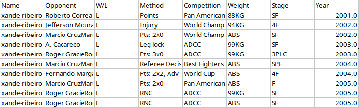
The majority of our features will come from the 'fighter_record' dataset, which, as shown above, includes the names of the two competitors, the match outcome (W/L), the method of victory, the competition, the weight class, and the year. In its current form, this data is unlikely to be highly predictive. However, we can extract more predictive features from this dataset, such as the win percentage of the fighters at the time of the match, the submission types that the fighters excel at and struggle to defend against, and the weight classes in which the fighters typically compete.
Creating the Explanatory Features
The first feature I want to create is the win percentage for the two competitors. Intuitively, a competitor with a 90% win percentage is expected to have a higher chance of winning against a competitor with only a 10% win percentage. Therefore, we need to perform some data manipulation to create a metric that compares the win rates of the two competitors at the time of the fight.
The second feature I would like to implement is a measure of the relative strengths and weaknesses of competitors in relation to various classes of submissions. For instance, if a leg lock specialist competes against someone with a history of susceptibility to leg locks, it is likely that the leg lock specialist would win the match.
Another potentially valuable predictive feature we can derive from this data is the relative weight classes of the athletes. Since athletes often compete in different weight classes and we don't have the exact weight data for the athletes at the time of competition, we will need to make some assumptions to include this as a feature in our dataset.
The last feature I want to include in the predictive model is the popularity measurement I collected earlier. People are naturally more interested in the better athletes, so this metric will likely have significant predictive power in our model.
In the code below, I aggregate and summarize the `fighter_record` dataset. In my summary dataset, I aggregate the data by the fighters' names and then summarize their wins and losses, including submission wins and losses. Submissions are grouped into three types: arm locks, leg locks, and chokes. I then connect the win information to the `Name` column and the loss information to the `Opponent_Lower` column.
The way I summarize the submission proficiency data is more simplified than I would like. While it provides a general understanding of fighters' proficiency in the three broad categories, I could likely achieve more predictive power by avoiding broad categorization of the submissions. Additionally, the number of wins and losses in this summary accounts for the entire careers of the competitors and does not reflect their records at the time of the competition. If I wanted to dive deeper into this analysis, I could improve these features by expanding upon these ideas.
Compare the Win Percentages of the Competitors by Submission Group
import pandas as pd
import re
import numpy as np

# Load the datasets
df_info = pd.read_csv('fighter_info.csv')
df_records = pd.read_csv('fighter_record.csv')
df_submission_types = pd.read_csv('submission_type.csv')

# Function to clean duplicated names
def clean_duplicated_names(name):
    if pd.isna(name):
        return name
    name = str(name)  # Ensure the variable is a string

    pattern = re.compile(r'^(.+?)(\1)+$')
    match = pattern.match(name)
    if match:
        return match.group(1).strip()
    return name

df_records['Opponent_Clean'] = df_records['Opponent'].apply(clean_duplicated_names)
df_records['Opponent_Lower'] = df_records['Opponent_Clean'].str.lower().str.replace(' ', '-')

# No filtering - use entire dataset
df_filtered = df_records.copy()

# Merge df_submission_types into df_filtered on the 'Method' column
df_merged = pd.merge(df_filtered, df_submission_types, how='left', on='Method')
df_merged['Sub_Type'] = df_merged['Sub_Type'].fillna('No Submission')

# Define relevant submission types
submission_classes = ['arm_lock', 'leg_lock', 'choke']

# Initialize the summary dictionary
summary_dict = {'Name': []}

# Add summary columns
summary_columns = ['Total_Wins', 'Total_Losses',
                   'Submission_Wins', 'Submission_Losses']

# Add columns for each submission type
for sub_class in submission_classes:
    summary_columns += [
        f'{sub_class.replace(" ", "_")}_Wins',
        f'{sub_class.replace(" ", "_")}_Losses',
        f'{sub_class.replace(" ", "_")}_Win_Rate',
        f'{sub_class.replace(" ", "_")}_Loss_Rate'
    ]

# Add additional columns to the summary dictionary
additional_columns = ['Submission_Win_Rate_Fighter', 'Total_Win_Fighter', 'Submission_Win_Opponent', 'Total_Win_Opponent']
summary_columns += additional_columns

# Initialize the dictionary with all required columns
for col in summary_columns:
    summary_dict[col] = []

# Function to compute the summary stats for a fighter
def compute_summary(name, group):
    total_wins = group[group['W/L'] == 'W'].shape[0]
    total_losses = group[group['W/L'] == 'L'].shape[0]
    submission_wins = group[(group['W/L'] == 'W') & (group['Sub_Type'] != 'No Submission')].shape[0]
    submission_losses = group[(group['W/L'] == 'L') & (group['Sub_Type'] != 'No Submission')].shape[0]

    summary = {
        'Total_Wins': total_wins,
        'Total_Losses': total_losses,
        'Submission_Wins': submission_wins,
        'Submission_Losses': submission_losses,
    }

    for sub_class in submission_classes:
        sub_wins = group[(group['W/L'] == 'W') & (group['Sub_Type'] == sub_class)].shape[0]
        sub_losses = group[(group['W/L'] == 'L') & (group['Sub_Type'] == sub_class)].shape[0]

        summary[f'{sub_class.replace(" ", "_")}_Wins'] = sub_wins
        summary[f'{sub_class.replace(" ", "_")}_Losses'] = sub_losses
        summary[f'{sub_class.replace(" ", "_")}_Win_Rate'] = (sub_wins / submission_wins) if submission_wins > 0 else 0
        summary[f'{sub_class.replace(" ", "_")}_Loss_Rate'] = (sub_losses / submission_losses) if submission_losses > 0 else 0

    # Add computed win rates
    summary['Submission_Win_Rate_Fighter'] = submission_wins / total_wins if total_wins > 0 else 0
    summary['Total_Win_Fighter'] = total_wins
    summary['Submission_Win_Opponent'] = total_losses / submission_losses if submission_losses > 0 else 0
    summary['Total_Win_Opponent'] = total_losses

    return summary

# Aggregate the data by fighter
for name, group in df_merged.groupby('Name'):
    summary_dict['Name'].append(name)
    summary_stats = compute_summary(name, group)
    for col in summary_columns:
        summary_dict[col].append(summary_stats[col])

# Create the summary DataFrame from the dictionary
df_summary = pd.DataFrame(summary_dict)

# Prepare Wins Summary DataFrame
win_cols = ['Name', 'Total_Wins', 'Submission_Wins'] + [f'{x.replace(" ", "_")}_Wins' for x in submission_classes] + [f'{x.replace(" ", "_")}_Win_Rate' for x in submission_classes]
df_wins_summary = df_summary[win_cols]

# Prepare Losses Summary DataFrame
loss_cols = ['Name', 'Total_Losses', 'Submission_Losses'] + [f'{x.replace(" ", "_")}_Losses' for x in submission_classes] + [f'{x.replace(" ", "_")}_Loss_Rate' for x in submission_classes]
df_losses_summary = df_summary[loss_cols]

# Merge wins summary data with df_filtered['Name']
df_filtered_with_wins = df_filtered.merge(df_wins_summary, how='left', left_on='Name', right_on='Name')

# Merge losses summary data with df_filtered['Opponent_Lower']
# Rename the 'Name' column in df_losses_summary to allow merge with 'Opponent_Lower'
df_losses_summary = df_losses_summary.rename(columns={'Name': 'Opponent_Lower'})
df_final = df_filtered_with_wins.merge(df_losses_summary, how='left', on='Opponent_Lower', suffixes=('_fighter', '_opponent'))
The summarized data that I connect to my central data frame is essentially presented in the Shiny app below. You can toggle through this app to see the fighters' win and loss numbers, along with their relative wins and losses by submission type.
We can now move on to the code where I calculate the relative weight of the competitors. This dataset contains a string representing the various 'KG' weight classes in which the competitors participated, but it does not provide the actual weights of the fighters. To address this, I determine the weight classes the fighters competed in most frequently (the mode) and connect that to the central dataset. I then calculate the difference between the fighters' weight classes to use in my predictive model.
Compare the Relative Weight of the Fighters/h5>
# Filter out 'ABS' values (case insensitive)
df_records['Weight'] = df_records['Weight'].astype(str)  # Convert Weight to string
df_filtered_weights = df_records[~df_records['Weight'].str.contains('ABS', case=False, na=False)]

# Remove the 'KG' suffix and 'O' prefix
df_filtered_weights.loc[:, 'Weight'] = df_filtered_weights['Weight'].str.replace('KG', '', case=False).str.replace('O', '', case=False)

# Convert weight to numeric for mode calculation
df_filtered_weights.loc[:, 'Weight'] = pd.to_numeric(df_filtered_weights['Weight'], errors='coerce')

# Calculate the mode for each athlete
mode_weights = df_filtered_weights.groupby('Name')['Weight'].agg(
    lambda x: x.mode()[0] if not x.mode().empty else np.nan).reset_index()
mode_weights = mode_weights.rename(columns={'Weight': 'Native_Weight'})

# Merge mode weights back to the final DataFrame
df_final = pd.merge(df_final, mode_weights, on='Name', how='left')
df_final = pd.merge(df_final, mode_weights, left_on='Opponent_Lower', right_on='Name', suffixes=('', '_Opponent'))

# Drop redundant 'Name_Opponent' column
df_final = df_final.drop(columns=['Name_Opponent'])

# Calculate 'relative_weight'
df_final['relative_weight'] = df_final['Native_Weight'] - df_final['Native_Weight_Opponent']
David vs. Goliath size difference in match. Mackenzie Dern vs. Gabi Garcia 2017
Adding the Popularity Metric and Wrapping Things Up
The last feature I want to add is the difference in fighters' popularity levels, measured by the relative difference in the number of views on their profile pages. I expect this feature to have significant predictive power, as people tend to be more interested in fighters perceived as better performers. In the code below, I will incorporate the popularity metric and save the final dataset as a CSV file, which I can then upload in a separate script containing my predictive models.
# Encode 'W/L' column
df_final['Result_Coded'] = df_final['W/L'].map({'W': 1, 'L': 0})

# Calculate the '_metric' columns
for sub_class in submission_classes:
    wins_col = f'{sub_class}_Wins'
    loss_rate_col = f'{sub_class}_Loss_Rate'
    metric_col = f'{sub_class}_metric'

    df_final[metric_col] = df_final[wins_col] * df_final[loss_rate_col]

df_final['Win_Metric'] = df_final['Total_Wins'] - df_final['Total_Losses']
df_final['Sub_Win_Metric'] = df_final['Submission_Wins'] - df_final['Submission_Losses']

# Extract and rename relevant columns from df_info before merging
df_info_selected = df_info[['Name', 'Number']].rename(columns={'Number': 'Popularity_Fighter'})
df_info_opponent = df_info[['Name', 'Number']].rename(columns={'Name': 'Opponent_Lower', 'Number': 'Popularity_Opponent'})

# Merge df_info with df_final for fighters
df_final = pd.merge(df_final, df_info_selected, on='Name', how='left')

# Merge df_info with df_final for opponents
df_final = pd.merge(df_final, df_info_opponent, on='Opponent_Lower', how='left')

# Calculate 'Popularity_Difference'
df_final['Popularity_Difference'] = df_final['Popularity_Fighter'] - df_final['Popularity_Opponent']

def select_columns(df):
    columns = [
        'Name', 'Competition', 'Stage', 'Year', 'Opponent_Lower', 'Win_Metric',
        'Sub_Win_Metric', 'arm_lock_Wins', 'leg_lock_Wins', 'choke_Wins',
        'relative_weight', 'Result_Coded', 'arm_lock_metric', 'leg_lock_metric',
        'choke_metric', 'Popularity_Difference'
    ]
    return df[columns]

# Apply the function to select specific columns
df_final_selected = select_columns(df_final)

# Save the final DataFrame to a CSV file
df_final_selected.to_csv('final_data.csv', index=False)

# Display the final DataFrame to verify
print(df_final_selected.head())
Before saving my dataset for use in predictive models, I want to encode the 'W' and 'L' values in the 'W/L' column to show a 1 for a win and a 0 for a loss. Additionally, I will add a boolean column to indicate if the win was by submission, as a submission win is a much better indicator of the superior fighter compared to a win by points or decision. In the final step, I will select the columns to include in my predictive model and save the data frame. The dataset can be downloaded via the button below.
Now that we have a dataset with strong predictive features, we can proceed with building models and evaluating their performance. When creating predictive models, it is crucial to separate our dataset into training and testing sets to avoid overfitting. In addition to the standard train-test split process, we need to address the issue of having two entries for each match—one for each competitor. If we use simple randomization to split our data, we risk training our model with information that also appears in the test set.
In the following code, I split the dataset into training and testing subsets using the `train_test_split` function from the `sklearn` library. This function efficiently partitions the data into two groups. Since our dataset contains two rows for each match, I needed to account for this when splitting.
To achieve this, I created a `unique_matches` DataFrame that uses a combination of the competition, stage, and year columns to generate a unique identifier for each match. This unique identifier ensures the train and test splits can be reassembled accurately.
Split Data into Train and Test Sets
import pandas as pd
import numpy as np
from sklearn.model_selection import train_test_split, GridSearchCV
from sklearn.linear_model import LogisticRegression
from sklearn.ensemble import RandomForestClassifier
from sklearn.metrics import accuracy_score, precision_score, recall_score, f1_score, confusion_matrix
from sklearn.preprocessing import StandardScaler

# Load the dataset
df = pd.read_csv('final_data.csv')

# Combine the columns to create a unique identifier for each match
df['match_id'] = (
    df['Competition'].astype(str) + '_' +
    df['Stage'].astype(str) + '_' +
    df['Year'].astype(str)
)

# Drop rows where Result_Coded is NaN
df = df.dropna(subset=['Result_Coded'])

# Verify the shape after dropping NaNs
print('Shape after dropping NaNs for Result_Coded:', df.shape)

# Get the unique matches
unique_matches = df[['match_id']].drop_duplicates()

# Verify unique matches
print('Number of unique matches:', unique_matches.shape[0])

# Split these unique matches into train and test sets
train_matches, test_matches = train_test_split(unique_matches, test_size=0.2, random_state=1234)

# Verify the split of unique matches
print('Training matches:', train_matches.shape[0])
print('Test matches:', test_matches.shape[0])

# Filter the original DataFrame to create train and test sets based on match_id
train_set = df[df['match_id'].isin(train_matches['match_id'])]
test_set = df[df['match_id'].isin(test_matches['match_id'])]

# Verify the shape of the training and testing set after filtering
print('Training set shape after filtering:', train_set.shape)
print('Testing set shape after filtering:', test_set.shape)

# Drop the temporary match_id column
train_set = train_set.drop(columns=['match_id'])
test_set = test_set.drop(columns=['match_id'])

# Drop the 'Year' column from both train_set and test_set
train_set = train_set.drop(columns=['Year'])
test_set = test_set.drop(columns=['Year'])

# Verify the split
print('Train set info:')
print(train_set.info())
print('Test set info:')
print(test_set.info())

# Features and target
X_train = train_set.drop(columns=['Result_Coded'])
y_train = train_set['Result_Coded']
X_test = test_set.drop(columns=['Result_Coded'])
y_test = test_set['Result_Coded']

# For simplicity, we will only use numeric features for logistic regression and random forest
# You might need further preprocessing for categorical features if any
numeric_features = X_train.select_dtypes(include=[float, int]).columns

X_train = X_train[numeric_features]
X_test = X_test[numeric_features]

# Verify the numeric features
print('Numeric features:', numeric_features)

# Handling missing values by filling them with the median
X_train = X_train.fillna(X_train.median())
X_test = X_test.fillna(X_test.median())

# Ensure there are no infinite values (replace them with large finite numbers)
X_train = X_train.replace([np.inf, -np.inf], np.nan).fillna(X_train.median())
X_test = X_test.replace([np.inf, -np.inf], np.nan).fillna(X_test.median())

# Standardize the numeric features
scaler = StandardScaler()
X_train = scaler.fit_transform(X_train)
X_test = scaler.transform(X_test)

# Verify no NaN or infinite values in y
y_train = y_train.fillna(0)
y_test = y_test.fillna(0)

# Check the final shapes and value counts
print('Final training set shape:', X_train.shape, 'Target shape:', y_train.shape)
print('Final test set shape:', X_test.shape, 'Target shape:', y_test.shape)
print('Training target value counts:', y_train.value_counts())
print('Testing target value counts:', y_test.value_counts())
Now that I have my training set, I can begin training models suitable for binary classification, such as logistic regression and decision trees. In the code below, we will set up a basic logistic regression model.
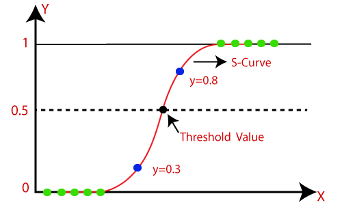
Logistic regression is a statistical method used for binary classification problems, where the outcome variable can take on one of two possible values. It models the probability that a given input point belongs to a particular class. The logistic regression function is defined using the logistic (sigmoid) function to map predicted values to probabilities between 0 and 1, making it ideal for binary outcomes. The chart below provides a quick visualization of how probability values are mapped to binary outcomes.
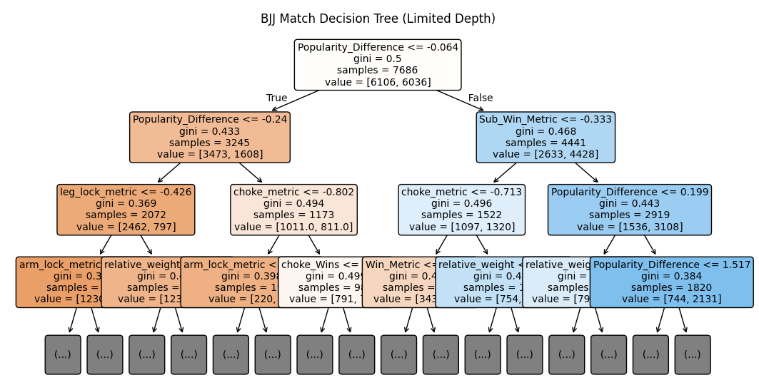
We will now evaluate whether a decision tree model can enhance basic performance. Decision trees are commonly utilized for classification tasks as they systematically divide a dataset into subsets according to the features of the data. The algorithm iteratively splits the dataset, forming groups based on the predictive power of each feature. These divisions result in a series of branches that collectively give the decision tree its distinctive tree-like structure, as illustrated in the plot below.
BJJ Competition Decision Tree
In this example, I employ a random forest algorithm to implement an ensemble of decision trees and select the most effective model. The code for this process is shown below.
      # Random Forest Classifier
print("\nRandom Forest Model with Hyperparameter Tuning:")
rf_param_grid = {
    'n_estimators': [50, 100],
    'max_depth': [10, 20, None],
    'min_samples_split': [2, 5]
}
rf_model = RandomForestClassifier(random_state=1234)
rf_grid_search = GridSearchCV(rf_model, rf_param_grid, cv=5)
rf_grid_search.fit(X_train, y_train)

best_rf_model = rf_grid_search.best_estimator_

# Make predictions on the test set
y_pred_rf = best_rf_model.predict(X_test)

# Calculate evaluation metrics
accuracy_rf = accuracy_score(y_test, y_pred_rf)
precision_rf = precision_score(y_test, y_pred_rf)
recall_rf = recall_score(y_test, y_pred_rf)
f1_rf = f1_score(y_test, y_pred_rf)
conf_matrix_rf = confusion_matrix(y_test, y_pred_rf)

# Print the evaluation metrics
print(f'Accuracy: {accuracy_rf:.2f}')
print(f'Precision: {precision_rf:.2f}')
print(f'Recall: {recall_rf:.2f}')
print(f'F1 Score: {f1_rf:.2f}')
print('Confusion Matrix:')
print(conf_matrix_rf)

# Print feature importances for Random Forest
rf_importances = pd.DataFrame({'Feature': numeric_features, 'Importance': best_rf_model.feature_importances_})
rf_importances = rf_importances.sort_values(by='Importance', ascending=False)
print("\nRandom Forest Feature Importances:")
print(rf_importances)

# Control the Max Depth (restricts how deep the visualization goes)
# Beware, it's restricting visualization, not tree pruning based purely on features.
tree_to_plot = best_rf_model.estimators_[0]

# Visualize specified depth
plt.figure(figsize=(20, 10))
plot_tree(tree_to_plot, max_depth=3,  # Adjust depth here. Smaller values make simpler plots.
          feature_names=numeric_features, filled=True, rounded=True, fontsize=10)
plt.title("BJJ Match Decision Tree (Limited Depth)")
plt.show()
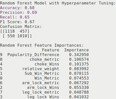
As shown in the confusion matrix metrics in the image below, this predictive model demonstrates a similar level of predictive capability to the logistic regression model used previously.
Random Forest Model Behaivor
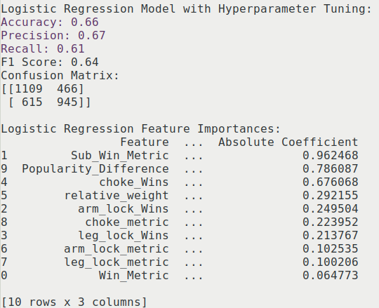
While this model exhibits predictive capabilities similar to the logistic regression model, the relative importance of features differs significantly. In the logistic regression model, the most predictive factor is the difference in win and loss rates between competitors, followed by their popularity. Conversely, in the random forest model, popularity is the most influential feature. Interestingly, the relative weight of the competitors did not hold as much predictive power as anticipated. This may be because matches outside of the natural weight classes are often specifically chosen, frequently due to the exemplary performance of the smaller athlete.
Conclusion
To enhance the practical value of this model beyond a basic data science exercise, significant improvements are necessary to increase its predictive power. Currently, the model achieves approximately 66% accuracy, which is only marginally better than a random prediction with a 50:50 baseline. To enhance predictive accuracy, the primary focus should be on refining the features. The submission types were simplified into broad categories, which may not effectively capture my hypothesis: that we can identify athletes proficient in specific submission types and predict their success against opponents who have previously been defeated by those submissions.