The Fractional Factorial Design

Fractional factorial designs provide an excellent starting point for research. The design structure allows researchers to explore a vast design space with a relatively small number of runs. Although these designs require more runs than minimal screening experiments, they can, when executed correctly, help researchers identify both the critical factors that influence the response and the interactions between those factors. In this blog post, I will present an example of a fractional factorial design I conducted in R, followed by a detailed discussion of the essential aspects to consider when using R for this type of experiment.

Avocado Tissue Culture

Over the past year, a significant portion of my work has focused on developing a tissue culture system for avocados. Currently, the demand for avocado trees is met through clonal propagation in greenhouses, which is costly, relies on seasonal materials, and is time-consuming. Developing a tissue culture platform for a wide range of avocado varieties could revolutionize the market supply chain by reducing production costs and enabling the availability of an unlimited number of plants.

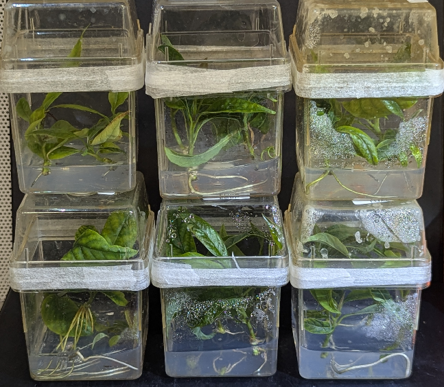
Although it took some time to reach this stage, the picture below, which shows avocado clones in the rooting phase of tissue culture, demonstrates our substantial success in developing a platform for avocado production.

It required significant research to enable Tissue-Grown Corporation to produce avocado tissue cultures with such effective performance. No tissue culture lab has successfully achieved a commercial-scale propagation system for avocados, as they are notoriously difficult to culture using modern methods.

Tissue-Grown's initial attempts at culturing this plant encountered common issues frequently reported in the literature. The plants would grow initially, but then the leaves would start to fall off and the cultures would turn black. During this process, the growth rate of the apical meristem would slow until the cultures ultimately failed.

Being early in the process development, this was an opportune time to perform a factor screen. The goal was to identify the chemical and environmental factors that would enable the plant to survive and thrive in culture.

A Brief Introduction to the Fractional Factorial Design

Before delving into my specific use case, let's review the basics of how factorial designs works. All factorial designs require each potential factor to be tested at two levels. The primary objective is to determine if there is a difference in performance between the runs at the low level and the high level of the factor. In a full factorial design, a researcher would need one run for every possible combination of the two levels for each factor.

While this design is excellent for testing a small number of factors, it quickly becomes impractical for screening a large number of factors. For example, testing eight factors would require 2^8 (128) runs. This is where the fractional factorial design excels. If a researcher is not interested in every possible interaction within the design space, it is not necessary to include every potential run in the experiment.

In a fractional factorial design, a researcher can specify the level of interactions they are interested in and reduce the required design size accordingly. The picture below provides a color-coded explanation of the design resolutions. These different resolutions indicate what level of interactions can be discerned from the design, based on the number of factors and the number of runs.

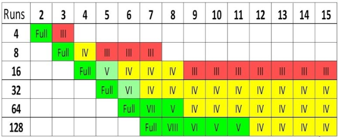
Fractional Factorial Design Resoltion Chart from StatEase

Design Resolution Numbers Explained

• Full Factorial Design: all combinations are tested for all factors. This design can identify all potential interactions.
• Resolution III: no main effects are aliased with other main effects, but the main effects are aliased with two-factor interactions. This design requires the least number of runs, but should not be used to evaluate interactions.
• Resolution IV: no main effects are aliased with any other main effect or 2-factor interactions, but some 2-factor interactions are aliased with other 2-factor interactions and main effects are aliased with 3-factor interactions. This design is normally sufficient to identify all of the main factors and two-factor interactions in a design.
• Resolution V and Higher: no main effects or two-factor interactions are aliased with main effects or two-factor interactions, but the two-factor interactions can be aliased with higher-order interaction.

Understanding how design resolutions work helps me choose the appropriate design size for my experiment. While individual interactions are rare, interactions among many factors in a complex system are common. Therefore, in the following experiment, I decided to use a Resolution IV design. This approach allows me to identify the main factors and, most likely, any two-factor interactions. Consequently, I opted for a 16-run, 8-factor design, which requires only 1/8 of the runs of a full factorial design.

I then make a list with eight factors that I want to include in my experiment and move forward with the design process.

Among the factors to be considered there will be the vital few and the trivial many.

Creating the Design in R

At this stage of the design process, I review the available research on the topic and compile a list of factors identified by others that affect my subject—in this case, the growth and survival of avocado tissue cultures. I combine my domain knowledge with insights gathered from online discussions to assemble a comprehensive list of components to test in my experiment.

Subsequently, I review the components and select eight to include in the Resolution IV design. For each factor in the experiment, I choose a high and low level, ensuring that the levels are set sufficiently apart to observe any potential effects. With my levels in hand, I can move forward creating the design in

How to Create the Design in R:

    
## Import the Packages I will use
library(tidyverse)
library(FrF2)

## Make sure to set the randomization so you can
## recreate the design at a later time
set.seed(1234)

##Import your working directory
##setwd("")

## Choose the 8 factors and create the design with the
## FrF2 function.
## Possible Factors:
## Cytokinin <- CPPU vs mT
## Cytokinin.Conc <- low vs. high
## Salt Mix <-  High CA 20 vs. V2G
## Glucose Level <- low vs high
## Extras (Casein, Glutamate, Ascorbic Acid) <- no vs yes
## Silver Nitrate <- low vs high
## Agar vs. Gelzan
## Gel Strength <- soft vs hard
					
design <- FrF2(16, 8, factor.names = list(
                          Cytokinin = c("CPPU", "mT"),
                          Cyt.Conc = c("low", "high"),
                          Salt.Mix = c("High.Ca.20", "V2G"),
                          Glucose = c(15, 35),
                          Extras = c("no", "yes"),
                          Silver.Nitrate = c(0.4, 4),
                          Gelling.Agent = c("Agar", "Gelzan"),
                          Gel.Strength = c("soft", "hard")))


## Save the design and make sure to comment it out.
## You want to be able to rerun the experiment later
## and not lose the data you actually used to perform
## the experiment.
#write_csv(design, "design.csv")

summary(design)

	  
  

The design summary below provides all of the information we need to get started with the design. If there were any concerns about the alias stucturing (i.e. the two-factor interations which will share an effect estimate), it would be easy to remake the design with a different generator.

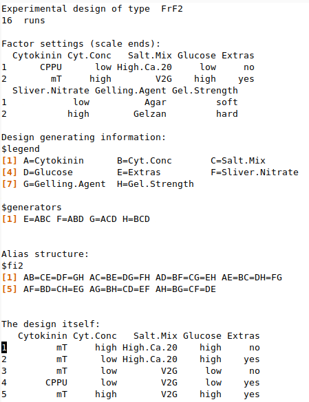
The FrF2 function from the FrF2 package easily creates as fractional factorial design with the indicated number of Runs, and Factor and is coded as indicated in the factor.names argument. With one this one function in R, you can easily create a fractional factorial design.

With the indended design built, I move forward with preparing the 16 different media for this project. I then initiated plants across the Runs and analyzed the growth performance characteristics after four weeks.

Analyzing the Results

After observing the plants in my trial, I measure as many potentially useful characteristics as I can identify. For this blog post, I will focus solely on the health of the apical meristem, as my primary goal in this project is to sustain active plant growth after initiation into a test tube.

As illustrated in the picture below, there is a substantial difference in the health of the apical meristem between the successful and unsuccessful runs in this experiment. When collecting data on the health of the apical meristem, I assign a value of 1 to plants with a healthy, growing tip and a value of 0 to those without. This data, along with other responses of interest, is recorded in a .csv file, which can be imported into R for analysis.

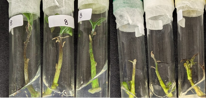
The difference in Tip Health Between the Good and Bad Runs in the experiment.

In the R code below, I import the design from the .csv file I saved earlier and the results from the .csv file where I recorded my results. I then perform some basic data aggregation with dplyr to summarize the results so I can then add them to the design I constructed with FrF2 with the add.response() function. With this completed, I can now visualize my results and then evaluate the statistical models.

Prepare the Results for Analysis:

    
## Import the design so there is less chance of the
## randomization seed changing the design structure.

des_import <- read_csv("design.csv") %>%
    mutate(Run = row_number())

## Results

results <- read_csv("results.csv")

results_summary <- results  %>%
    group_by(Run) %>%
    summarize(Quality = mean(Quality),
              Necrotic = mean(Necrotic),
              Shoots.per.Plant = mean(Total.Tips),
              Active.Apex = mean(Apical.Healthy),
              Plants.in.Exp = length(Run))

## Add the Summarzied Results to the Design

Response <- results_summary$Active.Apex

results_response <- add.response(design, Response)
	  
  

The first step in analyzing a factorial design is identifying the critical factors that control the majority of the response. My preferred visualization tool for this purpose is the half-normal plot. This plot allows for easy identification of the most influential factors by plotting the absolute value of the effect size against the theoretical quantiles.

In a half-normal plot, most factors will form a roughly straight line at the bottom left. The influential factors are easily distinguished because they deviate significantly from this line. Thus, it is straightforward to identify the factors controlling our response by finding the points farthest to the right that have deviated from the linear, best-fit line formed by the non-influential factors.

The `FrF2` library provides the easy-to-use `DanielPlot()` function to create this plot.

The Half-Normal Plot:

    
## A Half Normal Plot
DanielPlot(results_response, alpha = 0.4, half = TRUE)
	  
  

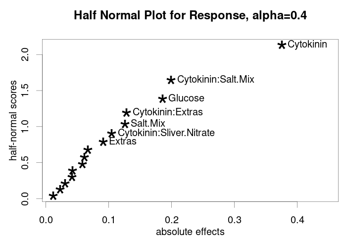
In this plot, it is immediately evident that cytokinin has a major effect on the health of the apical tip, as it significantly deviates from the line formed by the non-influential factors at the bottom left. While cytokinin is clearly the leading factor controlling our response, it is also possible that several other factors, including interactions, could be impactful, as they show some deviation from the best-fit line created by the non-influential factors. In the code above, I vary the alpha value to include more labels on the plot.

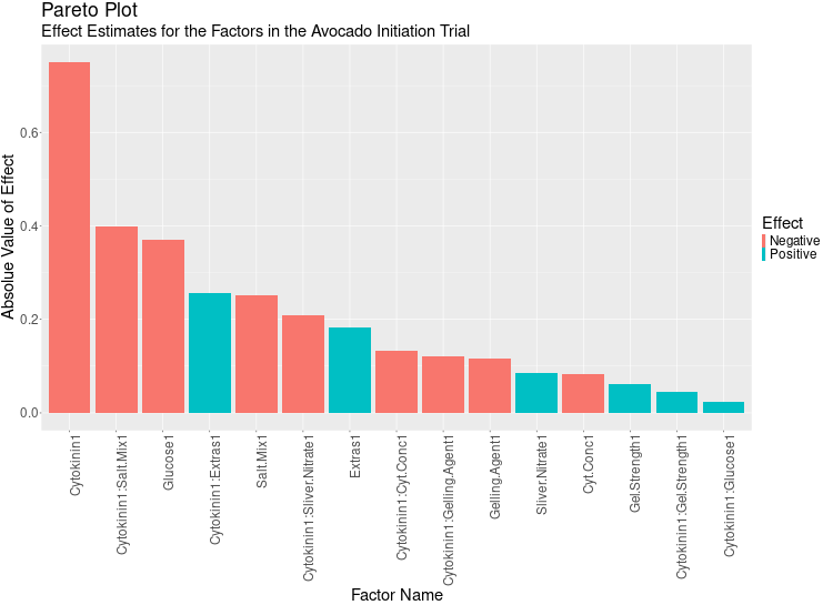
Another tool used to identify important factors in an experiment is the Pareto Plot. While the `FrF2` package does not include this feature by default, it can be easily created with a small amount of R code. The Pareto Plot is essentially a bar chart that displays the absolute values of effect sizes on the Y-axis and the effect names on the X-axis. In R, it is straightforward to extract the effect sizes from the output of the `lm()` function, as demonstrated in the code below. I then recreate the plot using `ggplot2`.

The Pareto Plot:

    
## Creating a Pareto Plot
mod.all <- lm(data = results_response, Response ~ (.)^2)


effect_df <- tibble(Names = names(mod.all$effects),
                    Values = mod.all$effects) %>%
    mutate(Abs.Value = abs(Values),
           Effect = ifelse(Values >= 0,
                           "Positive",
                           "Negative")) %>%
    filter(Names != "(Intercept)")


pareto_plot <- effect.df %>%
    ggplot(aes(y = Abs.Value,
               x = reorder(Names, Abs.Value, desc),
               fill = Effect)) +
    geom_bar(stat = "identity") +
    theme(axis.text.x = element_text(angle = 90,
                                     hjust = 1)) +
    labs(title = "Pareto Plot",
         subtitle = "Effect Estimates for the Factors in the Avocado Initiation Trial",
         y = "Absolue Value of Effect",
         x = "Factor Name")

pareto_plot
	  
  

It is then easy to use the left-most factors in this plot to build your regression models in subsequent steps.

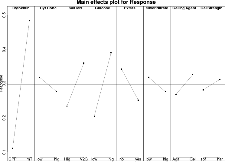
While we already have everything we need to construct our statistical models, I want to highlight two excellent charts we can create using the 'FrF2' package to demonstrate how the relevant factors influence our response: the main effects plot and the interaction plot.

The main effects plot displays the magnitude of the effects for the factors in a clear and concise manner, while the interaction plot shows how the interactions function. These two plots can be created with a single line of code, as shown in the code below.

Main Effect and Interaction Charts:

    
MEPlot(results_response)
IAPlot(results_response, select = c(1, 3, 5))
	  
  

In the main effects plot below, not only can you see the relative sizes of the effects of the factors in the design, but you can also obtain numeric results for the average response at the low and high levels in the design. From the half-normal and/or Pareto Plots, we know that the cytokinin choice was the single largest determinant of the response outcome. However, in this main effects plot, we can see that almost half of the plants in the experiment had active tips when the cytokinin was mT, whereas just over 10% had active tips when the cytokinin was 4-CPPU.

The interaction plot created with the `IAPlot()` function is tremendously useful for understanding how the factors in the design influence our response. In the plot below, I wanted to highlight the two strongest interactions in the experiment: cytokinin × salt mix and cytokinin × extras. When the cytokinin was 4-CPPU, there was almost no difference between the two salt mixes nor the inclusion of "extras" in the medium. However, when the cytokinin was mT, one salt mix performed significantly better, and the inclusion of extras negatively affected our response.

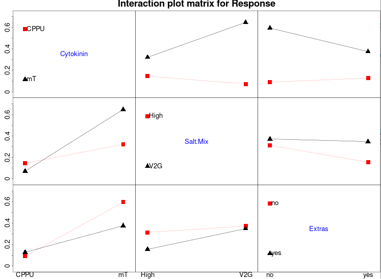
In this experiment, the interpretation of the interactions is straightforward and logical. When 4-CPPU was used as the cytokinin, the results were so poor that none of the other factors had any effect. However, in many cases, interactions can be confusing to interpret because the observed effect size is actually the sum of the highlighted interaction effect and three other aliased interactions. While it is not universally true, it is uncommon to observe interactions in a design when the main effect is not significant. Therefore, you can generally assume that the most significant main effects will be involved in the interactions.

If the interactions remain confusing, you can resolve this by folding the design. This process involves adding another set of runs to the experiment, which helps to clarify the aliasing. In this case, adding a fold to our 8 factor design .

Main Effect and Interaction Charts:

    
## Folding the Design:
folded_design <- fold.design(design)

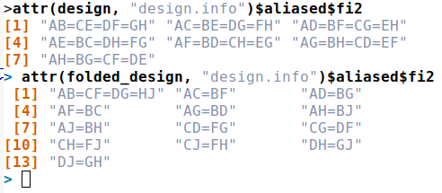
attr(design, "design.info")$aliased$fi2
attr(folded_design, "design.info")$aliased$fi2
	  
  

If the interactions remain confusing, you can resolve this by folding the design. This process involves adding another set of runs to the experiment, which helps to clarify the aliasing. In our case, folding the 8-factor design and increasing the number of runs from 16 to 32 does not increase the resolution number of the design. However, instead of having the critical interactions aliased with three other factors, most are only aliased with one.

We now have a clear understanding of the critical factors in our design and can construct statistical models to evaluate how well they fit our data.

Construct our Statistical Models

I will now create two separate statistical models from my data and evaluate their performance. The first model will include only our most significant factor, mT. The second model will include additional factors to determine how much more variation in our response is explained by the additional factors.

The statistical model with our only our most important response is created with the R code below.

Statistical Model with Only Main Effect:

    
## Statistical Model with Only the Main Effect
mod_1 <- lm(data = results_response,
            Response ~ Cytokinin)

summary(mod_1)
	  
  

The `summary()` function produces output like the one below, where you can see the p-values for the effects and the R-squared value, which measures how much variation in our model is explained. It is important to note that the t-values in the design summary are not appropriate in this instance, and we should be using analysis of variance to record the F-values.

I can easily convert my regression model to the appropriate ANOVA using the `car` package. Due to the loss of several runs in this experiment, it is necessary to use Type III ANOVA to account for the unbalanced design.

Comparing an ANOVA:

    
libary(car)

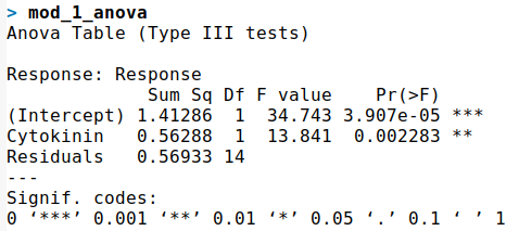
mod_1_anova <- Anova(mod_1, type = "III")

mod_1_anova
	  
  

As you can see in the ANOVA results, the t-values are appropriately converted to F-values, but the p-values remain largely the same. While it is technically correct to use analysis of variance in these types of experiments, I usually rely on the p-values from the `lm()` summary for my hypothesis testing as it requires less code.

Now, I will construct a statistical model using all the factors that showed any deviation in my half-normal plot. When adding new factors to my models, I evaluate whether the additional factors increase the amount of variation explained. The model summary provided by R includes a useful feature called the Adjusted R-squared, which accounts for the fact that adding factors will inherently increase the explained variability. Therefore, I evaluate whether adding more factors increases the Adjusted R-squared in the model summary.

Adding Model Terms:

    
## Statistical Model 2

mod_2 <- lm(data = results_response,
            Response ~ Cytokinin +
                Cytokinin:Salt.Mix +
                Glucose +
                Salt.Mix +
                Cytokinin:Extras +
                Cytokinin:Silver.Nitrate+
                Extras+
            Silver.Nitrate)

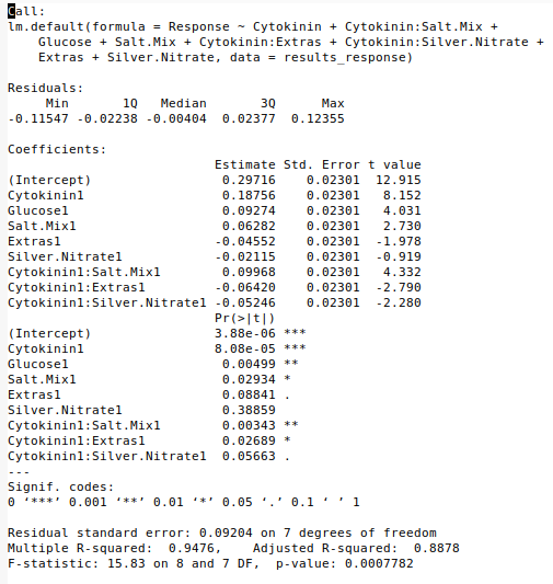
summary(mod_2)

	  
  

The addition of extra terms increases the Adjusted R-squared of my model from 0.46 to 0.89. Therefore, I will assume that factors other than cytokinin do indeed have an impact on my response and should be considered for future evaluation.

Summary

We have now completed the design and analysis of a fractional factorial design using R. Based on these results, I can create a new medium with the preferred levels of all significant factors and test it in an A/B comparison with my previous best-performing medium. In addition to improving the process, I can use these significant factors in future optimization research.

While this blog post was not intended to provide a detailed explanation of the fractional factorial design, I hope it demonstrates how easy it is to construct and analyze this type of design using R. Thanks so much for reading this post. If anyone has any questions or comments about this work, please feel free to email me.