Process Optimization with Response Surface Methodology
Once the primary factors controlling your response are identified, multiple linear regression can be employed to model the system's response to various inputs in an experiment. Such experiments necessitate testing multiple levels for each factor, which can result in sizeable experimental designs when several factors are involved. Response Surface Methodology (RSM) offers a framework to maximize the informational yield using the minimal number of experimental iterations. In this post, I will use R to create a specific RSM design—the Central Composite Design (CCD)—to optimize the in vitro rooting process of walnut plants.
Walnut Tissue Culture
Several years ago, my company received a large order for a specific walnut clone, Chandler. Although micropropagation methods for various walnut varieties were well-documented and effective in-house, this particular variety failed to form roots, rendering it unsellable. As a result, I was tasked with developing a method to induce rooting in these walnut cultures to ensure the success of the project.
I had previously conducted a highly successful factor screen experiment, which revealed that sucrose levels in the induction medium and incubation time were critical factors influencing the rate of root development during the root expression stage. Given that experimental runs in tissue culture are relatively inexpensive, I decided to include a rooting hormone (auxin) along with these two critical factors in my investigation. Consequently, I aimed to proceed with a three-factor optimization experiment to determine the optimal combination of these factors for maximizing the rooting rate.
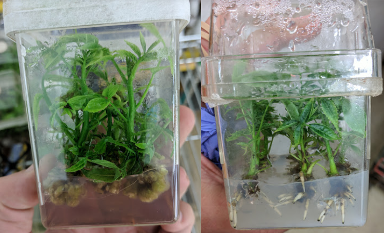
Walnut (Chandler) Cultures in Multiplication and Rooting.
In tissue culture, the rooting rate is a critical parameter influencing product cost. Each culture that meets the morphological requirements to enter the rooting stage incurs production expenses. If the rooting rate approaches zero, the product cost trends towards infinity. Therefore, developing an efficient rooting protocol is essential for minimizing product costs.
The Central Composite Design
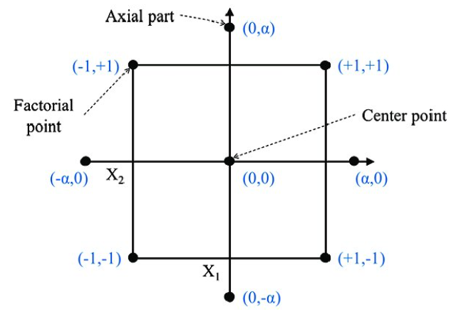
The foundations of experimental design are deeply rooted in geometry. While the geometry taught in school predominantly focuses on two-dimensional and three-dimensional shapes that we can visualize, experimental design requires the flexibility to explore higher-dimensional spaces, with each explanatory variable representing one dimension.
To sample the design space, the central composite design employs a circle (2D), sphere (3D), hypersphere (4D), and so forth, with most points concentrated toward the center of the geometric shape. It is a common practice to repeat the center point in these designs to gauge in-sample variation. The design also includes two points, known as factorial points, spaced equidistantly in both directions from the center for each explanatory variable. Additionally, two points called axial points are placed farther out to make the design rotatable, like a circle or sphere.
It is important to note that there is a specific class of CCD called a "face-centered design," where the axial points are the same distance from the center point as the factorial points. This design forms a square, cube, tesseract, and so on, rather than a round shape. It maintains many of the desired geometric properties of the rotatable CCD but is sometimes easier to use when the extreme levels of the axial points are impractical.
A visual explanation of the central composite design is shown in the figure below.
Another interesting attribute of the central composite design is that it can be built from previous factorial designs. If a previous screening experiment was conducted, the experimenter can use the levels from the previous factorial design as the factorial points, and then fill in the center and axial points in a subsequent experiment.
Building our CCD using R
Now, we will create a central composite design using R. As previously mentioned, our design will contain three factors: Incubation Time (in weeks), Sucrose (in g/L), and the rooting hormone IBA (mg/L). In the R code below, I will create the design using the `ccd()` function from the `rsm` package and visualize the resulting design.
Create a Central Composite Design in R:
## Import necessary libraries
library(rsm)
library(tidyverse)

## Set randomization seed so you can come back to exp.
set.seed(1234)

## Set working directory so it is easier to save/import
## setwd("\set_to_your_working_directory")

##create a central composite design with sucrose, time, iba
design <- ccd(3, n0 = 3,
              coding = list( x1 ~ (IBA - 5.5) / 2.5,
                             x2 ~ (Sucrose - 45) / 15,
                             x3 ~ (Time - 2) / 1),
              oneblock = TRUE)

## Convert Design in a Dataframe
design.decoded <- decode.data(design)

## Visualize the Design
design.plot <- design %>%
  decode.data() %>%
  ggplot(aes(y = Time, x = Sucrose, color = IBA)) +
    geom_jitter(width = 0.01,
                size = 10) +
    labs(title = "Central Composite Design",
         subtitle = "Rooting Experiment for Chandler Tissue Cultures",
         caption = "2D Representation",
         y = "Time (days)",
         x = "Sucrose (g/L)")

## Adjust Styling on Plot
design.plot +
    theme(legend.title = element_text(size = 13),
          legend.text = element_text(size = 8),
          legend.key.size = unit(5, "lines"),
          panel.background = element_rect(fill = "white", colour = NA),
          panel.border = element_rect(fill = NA, colour = "black"),
          panel.grid.major = element_line(colour = "grey80"),
          panel.grid.minor = element_line(colour = "grey90", size = 0.25),
          strip.background = element_rect(fill = "grey80", colour = "grey50"),
          strip.text = element_text(colour = "black"),
          plot.title = element_text(size = 16, face = "bold"))

## Save Design for Later Use
##write_csv(design.decoded, "design.csv")
The `ccd()` function handles most of the work in creating the design. In this function, we specify the number of variables (3), the number of center points (`n0 = 3`), and, using the `coding` argument, we define the names and levels of the explanatory variables. If the design is too large to complete in a single experiment, you may want to remove the `oneblock` argument.
The output from the `ccd` function is of the "coded-data" class and must be converted to a dataframe for normal analysis using the `decode.data()` function. Once the coded design is converted to a dataframe, it can be exported as a .csv file and visualized using `ggplot`.
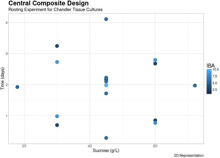
The plot created with `ggplot2` in the image below shows a 2D representation of the central composite design we created. I used `geom_jitter()` (instead of `geom_point()`) to clearly demonstrate that the center point is replicated multiple times and that 2^3 factorial points exist. Normally, the theme for the plot could be set with a single line of code using `+ theme_bw()`, but I wanted to change some attributes of the legend, so I fine-tuned it with the `theme()` function.
With the design completed, I can prepare the requisite media and conduct the experiment. For this experiment, I must label the media to indicate the incubation period and organize the process so that the plants are transferred from the root induction medium to the root expression medium at the appropriate time. After spending a specific amount of time in the expression medium, rooting rates will be collected and entered into a spreadsheet to begin the analysis process.
Analyzing the Results
With my results in hand, I can import the data into R and start visualizing it. In the R code below, I import my saved design and results, and then join them together based on the 'Run' column. Afterward, I use `ggplot2` to visualize the data.
Import the Results and Visualize:
results <- read_csv("results.csv")

des.import <- read_csv("design.csv") %>%
    rename(Run = run.order) %>%
    select(-std.order)

results.joined <- results %>%
	left_join(des.import, by = "Run") %>%
	select(-Run)

time.results <- results.joined %>%
    ggplot(aes(y = Rooting.Rate, x = Time, color = Sucrose)) +
    geom_jitter(width = 0.1,
                size = 10) +
    labs(title = "Longer Root Induction Periods Increase Rooting Rate",
         subtitle = "Rooting Results from Central Composite Design",
         caption = "Walnut Variety 'Chandler'",
         y = "Rooting Rate",
         x = "Incubation Time (weeks)")

time.results +
    theme(legend.title = element_text(size = 13),
          legend.text = element_text(size = 8),
          legend.key.size = unit(5, "lines"),
          panel.background = element_rect(fill = "white", colour = NA),
          panel.border = element_rect(fill = NA, colour = "black"),
          panel.grid.major = element_line(colour = "grey80"),
          panel.grid.minor = element_line(colour = "grey90", size = 0.25),
          strip.background = element_rect(fill = "grey80", colour = "grey50"),
          strip.text = element_text(colour = "black"),
          plot.title = element_text(size = 16, face = "bold"))
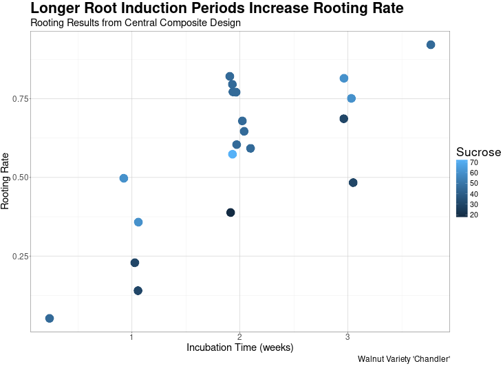
As you can see in the plot produced by the code above, the research was remarkably successful. It appears that there is a direct linear relationship between the incubation period and the rooting rate!
While this research indicates that we can achieve any desired rooting rate by extending the incubation period, it is still worthwhile to evaluate the performance of the other two explanatory variables, Sucrose and IBA. By analyzing our data, we can determine if optimizing these variables can further improve rooting performance. I will proceed by building some regression models to identify the optimal levels of these inputs.
Create Regression Models
## Build a Regression Model
## Simple Model with Time:
mod.1 <- lm(data = results.joined,
Rooting.Rate ~ Time)
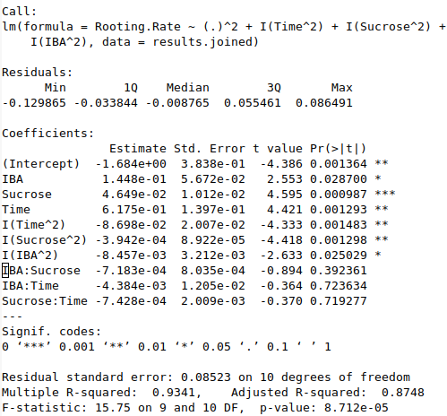
summary(mod.1) ## Model with time has R^2 of .571
## Full Model with All Terms:
mod.2 <- lm(data = results.joined,
Rooting.Rate ~ (.)^2 +
I(Time^2) +
I(Sucrose^2) +
I(IBA^2))
summary(mod.2) ## Adjusted R^2 of 0.875
The linear relationship observed in the plot above (Rooting Rate vs. Time) accounts for only around 57% of the variation in our data. By creating a full model that includes all possible first and second-order terms, along with their interactions, the adjusted R-squared increases to 93%. This suggests that we can improve the rooting rate not only by increasing the incubation time but also by optimizing the sucrose and IBA levels. The summary from the full regression model of the central composite design is shown below.
With our model complete, we can predict the rooting rates at the optimal conditions determined by the experiment. For comparison, I have included the model predictions for the initial conditions we used before this research: 1 week of incubation, 3 mg/L IBA, and 20 mg/L sucrose. This comparison allows us to see the predicted rooting rates for both our previous method and the optimal conditions identified by the regression model.
Evaluate Model Predictions
## Compare Predictions for this Model:

## Create sequences in design space
iba.levels <- seq(1, 10, by = 0.1)
sucrose.levels <- seq(18, 72, by = 1)
time.levels <- seq(0.2, 3.8, by = 0.1)

## Create a dataframe with all options in design space
design.space <- expand.grid(IBA = iba.levels,
                            Sucrose = sucrose.levels,
                            Time = time.levels)

predictions <- design.space %>%
    modelr::add_predictions(mod.2, var = "Rooting.Rate") %>%
    tibble() %>%
    filter(IBA == 5.5 & Sucrose == 51 & Time == 3.2 |
           IBA == 3 & Sucrose == 20 & Time == 1)

predictions
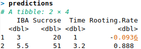
As shown in the model predictions above, the optimal rooting system produces significantly better rates than the system we used previously. However, it is noteworthy that the model predicted a rooting rate of less than 0 in some cases. This highlights the fact that there are more suitable regression models for this type of data, where values are restricted between 0 and 1. The probability values in our regression model are meant for normally distributed numbers and are not appropriate for a rooting rate confined to the 0–1 range. For modeling data, like ours that is a continuous proportion, we can use beta regression as you will see in the following code.
Implement Beta Regression
## Perform Beta Regression to More Accurately Model Continuous Proportion data from 0-1.
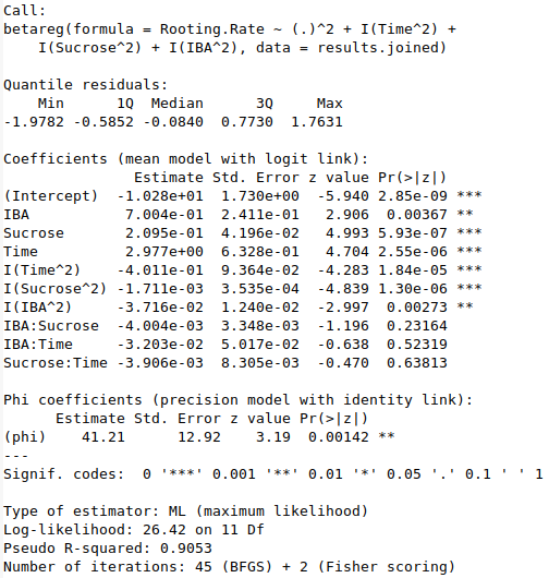
library(betareg)
mod.beta <- betareg(data = results.joined,
Rooting.Rate ~ (.)^2 +
I(Time^2) + I(Sucrose^2) + I(IBA^2))
summary(mod.beta)
From the summary of the beta regression model (below), we can see that the p-values are far more significant compared to those from the normal regression model. Additionally, the predicted outcome for our control process (IBA = 3, Sucrose = 20, Time = 1) is now a rooting rate of 0.055, instead of a negative value. The best predicted range is also extremely close to what we observed with the previous model. While the beta regression model is likely to produce more accurate predictions and p-values, it does not change the overall insights gained from this experiment.
All models are wrong, some are useful.
Conclusion
In this blog post, I presented an example of how to leverage response surface methodology for process optimization. Once an experimenter identifies the critical factors that control a response, it becomes relatively straightforward to design subsequent experiments aimed at determining the optimal levels of the explanatory variables. While deeper statistical understanding can lead to better predictive models, even a simple regression model (despite potentially inaccurate p-values) can still provide powerful explanatory insights.