Mixture Designs and TC Medium Mineral Optimization
One of the most challenging aspects of building tissue culture production systems is determining a suitable mixture of minerals for the plants. Every tissue culture system I have worked with can benefit from this type of research. However, it is almost impossible to conduct this research effectively without the appropriate Design of Experiment tools. In this post, I will demonstrate how to create mixture designs in R to address this problem.
Background: Plant Mineral Nutrition and Mixture Designs
Everyone who has practiced plant tissue culture is familiar with the Murashige and Skoog (MS) medium. The mineral salts in the MS medium have been a standard for micropropagation since the publication of the seminal paper, "A Revised Medium for Rapid Growth and Bio Assays with Tobacco Tissue Cultures," in 1962. This paper introduced a culture medium containing all the necessary macronutrients (N, P, K, Ca, Mg, S, and Cl) and micronutrients (Fe, B, Zn, Mn, Co, Cu, I, Mo, etc.). The MS salt mix is still widely used today. While it provides all the essential minerals for plant growth, it is not necessarily optimal. Almost every tissue culture can achieve superior results through mineral optimization.
While salt optimization is almost universally beneficial, very few tissue culturists attempt it because it requires advanced statistical tools. In this post, I want to demonstrate that salt optimization can be accomplished relatively easily through mixture experiments. Although these designs are more complicated to analyze than traditional regression models, efficient sampling of the design space can uncover superior results without requiring extensive statistical analysis. Often, selecting the best-performing run from a well-sampled design is sufficient to find a mineral mixture that significantly outperforms the controls. However, if data is available, it would be a missed opportunity not to use statistical methods to find the optimal result.
Creating Mixture Designs in R
In this post, I aim to introduce the audience to using mixture designs. I will demonstrate a straightforward approach to get started, which is particularly desirable due to the ease of media preparation. In a future post, I will discuss a different mixture design for optimizing the salt mixture in a tissue culture medium.
In this approach, I will create three concentrated salt mixes and blend them to efficiently sample the design space. While this method does not offer a theoretical understanding of how individual minerals impact culture growth, it can provide a high-performing salt mix for the experimenter.
In the R code below, I will use the `mixexp` package to create a mixture design with three different salt mixes. I will then duplicate this mixture space to test both high and low concentrations of the blends. This type of design is known as a mixture-process design, as it analyzes mixtures at two different levels.
Create a Central Composite Design in R:
library(mixexp)
library(tidyverse)
library(ggpubr)

set.seed(1234)

## setwd("set to your working directory")


## Define the three concentrates that will be used to create the blends
mix.comp <- c("Salt.Mix.1", "Salt.Mix.2", "Salt.Mix.3")

mixture.components <- length(mix.comp)

## Define the upper and lower ranges for the mixes.
lc <- rep(0.001, mixture.components)
uc <- rep(.998, mixture.components)

## This Xvert() function adds a point at all of the vertices
## and a center point.
salt.mix.perc <- Xvert(nfac = mixture.components,
                       lc = lc,
                       uc = uc)

## The Fillv() function fills the mixture space as evenly as possible
salt.mix.perc <- Fillv(nfac = mixture.components, salt.mix.perc)

colnames(salt.mix.perc) <- mix.comp

## Replicate the created blends at a high and low level
design.a <- salt.mix.perc %>%
    mutate(Salt.Strength = 0.5)

design.b <- salt.mix.perc %>%
    mutate(Salt.Strength = 1.5)

design <-rbind(design.a, design.b)

## Randomize the design and add Run numbers
design.random <- sample_n(design, size = nrow(design)) %>%
    mutate(Run = row_number())

##Write Design
##write_csv(design.random, "design.csv")

## Visualize the design
DesignPoints(salt.mix.perc, axislabs = mix.comp)
To create a mixture-process design in R, you need to define the upper and lower limits of the mixture space and add points to the extremes (vertices) using the `Xvert()` function. In our three-component design, this results in four points: one at each vertex of the triangle and the ternary blend in the middle. The `FillV()` function can then be used to evenly distribute additional points within the mixture design space. The first call to this function adds six points, but it can be called multiple times to increase sampling density. To transform the design from a mixture to a mixture-process design, we replicate the mixture at two levels. Finally, the design is saved for later use and visualized with the `DesignPoints()` function to create the output below.
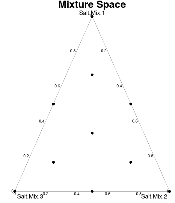
You can see in the ternary plot above that each point in our design consists of a blend of the three salt mixes. It is thus relatively easy to prepare the media by combining several stock solutions. Once the media is prepared, plants are worked on the medium and placed back into the growing environment for the desired incubation period. We are now ready to collect and analyze the results.
Analyze the Results
One major challenge in tissue culture research is appropriately quantifying the desired response variables. Some attributes, such as plant height or the number of shoots, are easily and consistently defined but may not directly correlate with success in culture. For instance, a very large plant may boost production rates in the early stages of a tissue culture system, but if the plants are not healthy, they are unlikely to perform well in downstream operations. Therefore, I often assign a Quality Score of 1-5 to each plant in the design for optimization purposes. While not ideal, I have found this to be a simple and effective method for optimizing culture systems.
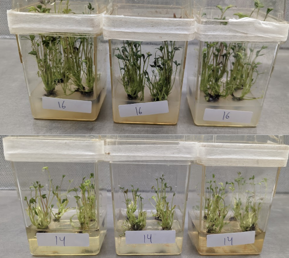
In these results, I will focus on some work I conducted with the beautiful flowering plant, the Peony. The picture below illustrates the differences observed between the better and worse performing runs. As you can see, the plants in the top picture are darker green and larger than those in the lower-scoring bottom picture.
In this design, we have two levels of the same experiment, allowing us to visualize whether better results were observed at the lower or higher level. In the code below, I import both the original design and the results, then merge them into a single dataframe for analysis. I create a quick visualization that shows better performance at the higher salt level in our design.
Import Results and Visualize
##Import Design and Results
results <- read_csv("results.csv")
des.import <- read.csv("design.csv")
## Join the Results and Design DataFrames
results.joined <- results %>%
left_join(des.import, by = "Run") %>%
mutate(Salt.Mix = case_when(Run %in% c(9, 14) ~ "Salt.Mix.1",
Run %in% c(12, 17) ~ "Salt.Mix.2",
Run %in% c(16, 18) ~ "Salt.Mix.3",
TRUE ~ "Blends"))
## Visualize Overall results with ggplot
results.joined %>%
ggplot(aes(y = Quality, x = Salt.Strength, color = Salt.Mix)) +
geom_jitter(width = 0.03, size = 20) +
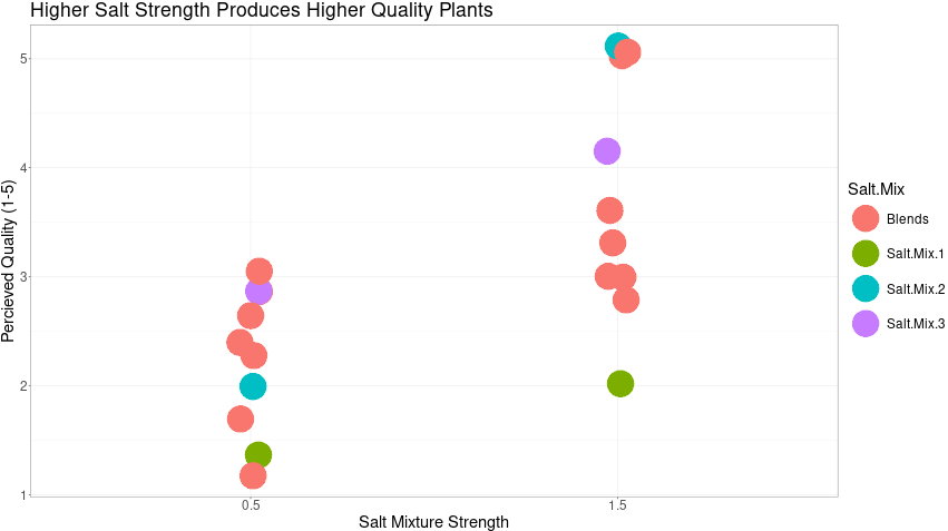
labs(title = "Higher Salt Strength Produces Higher Quality Plants",
y = "Percieved Quality (1-5)",
x = "Salt Mixture Strength") +
theme_bw()
As shown in the plot below, the higher salt strength blends resulted in higher quality plants.
In the next code section, we will use the analysis tools provided in the `mixexp` package to create a mixture regression model. The `MixModel()` function creates the regression model, and the `ModelPlot()` function provides a visualization of the model predictions. Since our model is a mixture-process type, we must set the `model` argument of the `MixModel()` function to type 5. You can find explanations for the model types in the help text for the `MixModel()` function.
Analyze with Mixture Tools
## Analyze results with tools from mixexp
results.joined$Salt.Strength <- as.factor(results.joined$Salt.Strength)
## Create the Model
## Model Type 5 is used for Mixture-Process
mixture.model <- MixModel(results.joined, "Quality",
mixcomps = c("Salt.Mix.1", "Salt.Mix.2", "Salt.Mix.3"),
procvars = "Salt.Strength",
model = 5)
## Visualize the Results
model.plot.low <- ModelPlot(model = mixture.model,
dimensions = list( x1 = "Salt.Mix.1",
x2 = "Salt.Mix.2",
x3 = "Salt.Mix.3"),
constraints = TRUE,
contour = TRUE,
fill = TRUE,
lims = c(0.01, 0.99, 0.01, 0.99, 0.01, 0.99),
axislabs = c("Salt.Mix.1", "Salt.Mix.2", "Salt.Mix.3"),
cornerlabs = c("Salt.Mix.1", "Salt.Mix.2", "Salt.Mix.3"),
pseudo = TRUE,
slice = list(process.vars = c(Salt.Strength = as.factor(0.5))),
colorkey = TRUE,
main = "Salt Strength 0.5x")
model.plot.high <- ModelPlot(model = mixture.model,
dimensions = list( x1 = "Salt.Mix.1",
x2 = "Salt.Mix.2",
x3 = "Salt.Mix.3"),
constraints = TRUE,
contour = TRUE,
fill = TRUE,
lims = c(0.01, 0.99, 0.01, 0.99, 0.01, 0.99),
axislabs = c("Salt.Mix.1", "Salt.Mix.2", "Salt.Mix.3"),
cornerlabs = c("Salt.Mix.1", "Salt.Mix.2", "Salt.Mix.3"),
pseudo = TRUE,
slice = list(process.vars = c(Salt.Strength = as.factor(1.5))),
colorkey = TRUE,
main = "Salt Strength 1.5x")
mix.plot <- ggarrange(model.plot.low,
model.plot.high,
nrow = 1)
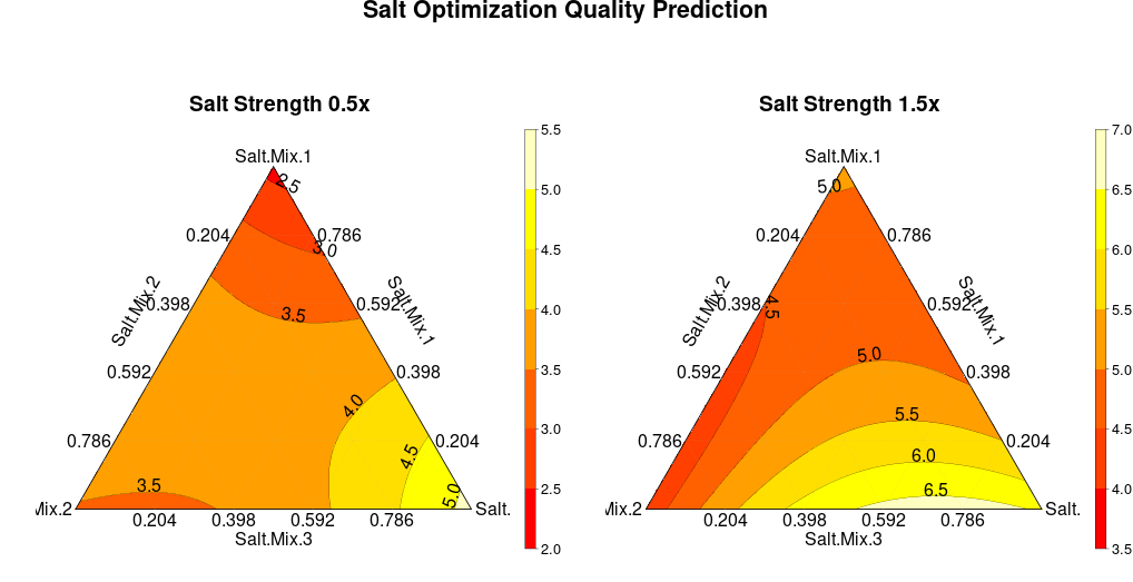
annotate_figure(mix.plot, text_grob(label = "Salt Optimization Quality Prediction",
face = "bold", size = 16))
I then use the `ggpubr` package to combine the two plots produced by `ModelPlot()` with `ggarrange()`. As you can see, the best results are predicted at approximately 75% Salt.Mix.3 and 25% Salt.Mix.1. This medium can then easily be reconstructed and tested in a future A/B test with controls.
Conclusion
This method demonstrates an easy-to-use approach for optimizing salt mixtures to improve the mineral nutrition requirements for plant tissue culture. Although it doesn't explain the behavior of the plants, it is useful because it is simple to conduct and samples the design space broadly. While this approach may not develop an optimal salt mixture, its broad sampling is likely to yield a mixture with superior performance compared to controls.
In this experiment, overall salt strength was a powerful indicator of plant quality. Since we only tested two levels for this variable, measuring the response curvature and finding an optimal level is impossible. This presents a great opportunity for a follow-up experiment focusing specifically on salt strength. With relatively few runs, there is a high likelihood of identifying a salt mix with superior performance.